Tutorial

1. Load spectra

Format of input data

MultiNMRFit requires that the main spectrum processing steps (baseline correction, phasing, …) have been performed beforehand. MultiNMRFit can load 1D NMR data provided in the following formats:

Pseudo2D: pseudo2D experiment (Bruker format only),

list of 1Ds: 1Ds spectra acquired independently (Bruker format only),

txt data: data from a tabulated text file (.txt extension) with the following structure:

ppm	0	…	n
0	1.2e3	…	1.2e6
0.1	1.3e3	…	4e7
0.2	2e8	…	3.6e3
…	…	…	…
12	3e4	…	7.85e3

The column ppm is mandatory and contains the ppm scale, columns named 0 to n correspond to each individual spectra and contain the intensities.

Note

list of 1Ds: The list of experiments should be provided as e.g.

1,8,109 : for non-consecutive spectra (here spectra 1, 8, and 109)
1-5 : for sequential spectra (here spectra 1,2,3,4,5)
1-5,109 : a mix of both formats for incomplete series (here spectra 1,2,3,4,5,109)

Inputs & outputs paths

data_path:: Path to the directory that contain the data
data_folder:: Folder containing your NMR data
expno:: List of Experiments which contain the spectra (i.e. expno in Topspin)
procno:: Process number (i.e. procno in Topspin)

Note

Inputs: The different fields will for inputs as described above will appear only for data type Pseudo2D & list of 1Ds. For txt data, the text file must be loaded using the drag-and-drop menu.

Note

procno: If a list of expno is provided the procno must be same for all expnos.

output_path:: Path to the folder use to export the outputs
output_folder:: Folder name
filename:: Name of the pickle file containing the process that will be automatically saved

Load a processing file

Current status of the process is continuously saved in a pickle file containing the entire process that has been perfomed. The pickle file can be reloaded using the drag-and-drop menu available in side bar of the Inputs & Outputs page.

2. Fit a spectrum

Once the data are correctly loaded the second page of the interface becomes available and allows users to fit one or several signals contained in a specific region of a given spectrum:

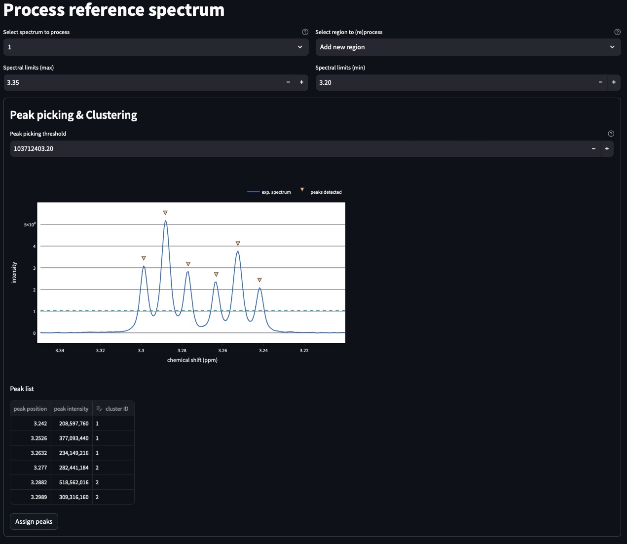
The top part of this page automatically performs peak picking on the reference spectrum within the region displayed in the plot:

Select spectrum: Select one the spectrum of the list.

Select region to (re)process: Multiple independent regions can be processed. Here, it will give you the possibility to display regions already processed or to define a new region to process.

Spectral limits (max): Maximal chemical shift of the spectral region (default is the maximum of the ppm scale)

Spectral limits (min): Minimal chemical shift of the spectral region (default is the min of the ppm scale)

Note

spectral limits: A region should be at least 0.025 ppm wide.

You can adjust the Peak picking threshold to detect the peaks of interest on the displayed spectrum.

While adjusting this threshold the software will automatically display a dataframe Peak list with the detected peaks in the region (marked with a yellow triangle on the spectrum). The peaks are displayed in the ascending order (e.g. from right to left on the spectrum). You can also add peaks mannually by entering their chemical shifts and click on “Add peak”.

You can now proceed with the clustering steps that consists in grouping peaks into a signal. For this purpose, fill the cluster ID column of the Peak list. Peaks that belongs to the same multiplets must have the same names.

Note

cluster ID: Signal IDs can be anything (numbers, strings, etc).

Once clustering has been performed, click Assign peaks to move towards the model construction step:

For each signal, MultiNMRFit will provide a list of all signal models that correspond to can be used (i.e. all signal models containing the corresponding number of peaks). You can also choose to add an offset, which corresponds to a first-order phase correction on the selected window. Once this step is done, you can click on Build model to automatically create the spectrum model and display the table of initial parameters.

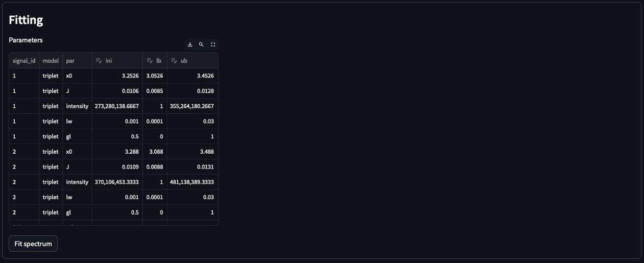
Initial values are calculated based on [i] the results of the peak picking (intensities and peak position) [ii] the default parameters of the each model (look at models.rst for more details on the default parameters). If no changes are required press the Fit spectrum button to fit the spectrum.

Note

Parameters: All parameters are shown in ppm units.

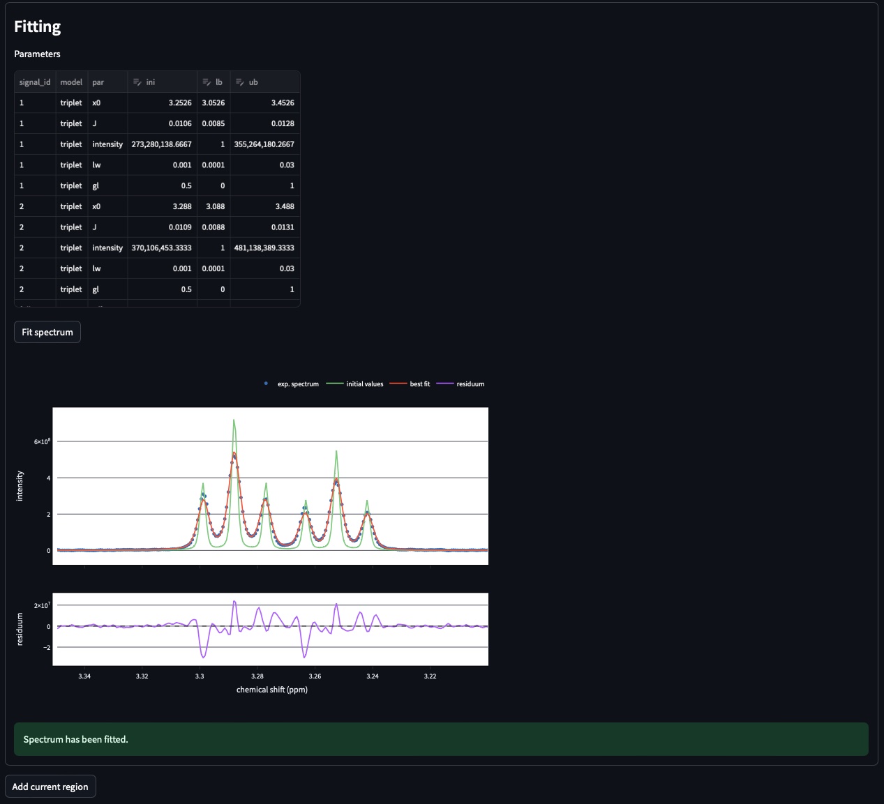
The fitted spectrum will be automatically displayed on the resulting plot. This plot shows [i] the experimental data as dots [ii] the best fit as red a curve and [iii] the initial values in green. The residuals plot (i.e. difference between the fitted and the experimental spectra) is shown below.

Note

Parameters: In the case of mismatch between the data and the best fit, you can adjust manually adjust the initial values in the former parameters table.

If the results are satisying, click on Add current region to save this region. To add another region, go to the top of page and select add new region in the field Select region to (re)process. Otherwise move to next page Fit from reference.

3. Batch analysis

This page contains the wrapper that enables fitting several spectra in batch based on an already processed spectrum (used as reference).

First select the region that you want to fit (Select region). MultiNMRFit will display the list of Signal IDs present in the selected region along with the processed spectra already analyzed.

Select the spectra you want to fit. By default it shows the complete dataset (here 1-256 as the pseudo2D contains 256 in the example). However if you want to analyze only the first ten spectra one can enter ‘1-10’ and MultiNMRFit will update the list spectra to process automatically. Click the Fit selected spectra to run the fitting of the selected spectra. The progress of the fitting will be displayed by a progress bar and once complete a message All spectra have been fitted will appear.

Note

Fitting: This procedure can be repeated for the different regions defined in the previous pages upon selection in Select region. By default MultiNMRFit do not reprocess spectra that have been already been fitted so clicked the option if necessary. The reference spectrum associated with the selected region can be visualized on this page.

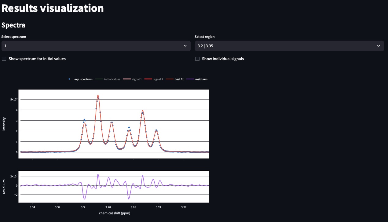
4. Results visualisation and export

This page enables visualizing the processing results in interactive plots. On top, you can inspect all fitted regions and spectra. If multiple signals were fitted on the same region, you can observe each one by clicking on the different signal IDs in the figure caption.

Spectra visualisation

Users can select the spectrum and the region to display.

Parameters visualisation

For the corresponding spectra shown above users can find the table of parameters. A particular attention must me given to the opt column that contains the values estimated from the best fit.

Finally, users can observe the change of a given paramters as function of spectra IDs.

Export results

Users can export their results tabulated text file in two different manners: all data or specific data In the first case (all data) all the parameters of all the regions and spectra will be saved in the output location defined in the first page of the interface. If the second case (option specific data selected), you can select one region, one parameter that will exclusively saved in the file.

Warning and error messages

Error messages are explicit. You should examine carefully any warning/error message. After correcting the problem, perform the analysis again.